My CFD archive

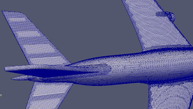
A rather unorthodox concept car geometry was chosen for automotive CFD analysis and the force Coefficients were calculated.  Figure No.1: STL geometry Turbulence properties were calculated from the wheel base length of the car and the Aerodynamic coefficients were calculated from the frontal area of the car. Here are the steps adhered to calculate the frontal area of the car using paraview. Here is a brief video tutorial on how to calculate the projection Area or the frontal area of a car.   The projection area and the wheelbase length values are called inside the force-coefficient file, within the system folder.  Figure No.2: lRef (base length) & Aref (Projection Area) The simulation was performed on a grid whose dimensionless wall-distance value was less than 1.0. A kOmegaSST turbulence model was adopted for a steady-state solver.  Figure No.3: Meshed STL geometry Along with the car, the ground patch or the lowerWall is also considered a

Before I begin to furnish the results, a quick look at the computational resources that were utilized for the simulation. I possess a minimal capability laptop manufactured by Hewlett-Packard, which runs on 2 core(s) and a 4 GB RAM. The objective of the simulation is to set up a 3D mesh for an Aircraft flow simulation with a resolved boundary layer of Y+ < 1, and to study the Residuals . The kOmegaSST turbulence model was adopted. The STL file downloaded online is a scaled Boeing 747 model, with the elevator tabs deflected downwards. Figure No.1: Rear View The cell size in the blockMesh is 0.05, owing to the fact that a scaled 747 model was selected, otherwise a cell size of 0.5 can be executed for an un-scaled model. Regardless, any of the following cell size can be applied (0.1, 0.2, 0.3, 0.4, 0.5, 0.6, 0.7, 0.8, 0.9, 1.0). Four boundary layers were generated with an expansion ratio of 1.2,  adding to the total cell count of over 3 million cells. A steady-state solver

This script is an adaptation of the original script written by Dr. Nguyen Vinh Tan, Agency for Science, Technology and Research, Singapore.  A matlab script with (.m) extension can be adopted from the following formula and the same can be run using mathwork or octave o n the linux platform. The turbulence properties and mesh layer thicknesses can be predicted using the same.  rho=1000; %This is density, a value 1.225 for air can be assigned nu=1.0e-6; %kinematic viscosity for air/water L=0.5; %L is the wheelbase length of a car/length of a flatplate/diameter for a cylinder simulation % If the reynolds number is assigned and the flow velocity has to be found out use: ReL = 60000; %global reynolds number Va = ReL*nu/L %If the flow velocity is assigned and the Reynolds number has to be calculated use: Va = 30; ReL = Va*L/nu %Turulence intensity can either be assigned or calculated I = 0.02; % 2 percentage(assigned) I = 0.05; % 5 percentage(assigned

The geometry chosen for external fluid dynamics simulation is that of an offshore structure. In that, a deep-draft semi-submersible structure  is scaled scaled down to a value  of 0.01 (scaled down by a factor of 100). The semi-submersible structures are employed at locations where the oil extraction from the sea bed is considerably deep. These are movable structures which are half submerged during application. A working deck comes right on top of the structure where the cranes and oil rigs are fitted. The semi-submersible consists of four hull appendages which connect the working deck with a pontoon structure. The pontoon structure gives buoyancy to the semi-submersible in deep waters but does not come directly in contact with the ocean bed.  Figure No.1: DDS The effects of flow induced vibration on the above four columns during high flow currents is indeed the case of interest. Once a good mesh is achieved, the platform is set for the study on the effects of Vortex Induced

Here are few results compiled from the Cylinder simulation. I have chosen the following Reynolds numbers for the study: 30, 200, 10000, 1*10^6.  Reynolds Number 30: Figure No.1: Flow Visualization  At a low Reynolds number of 30, the vortex shedding has not begun and so the force Coefficient of lift could not be calculated, as shedding is reason for the lift to exist. Reynolds Number 200: Figure No. 2: Force Coefficient & Strouhal number For a Reynolds number of 200, the vortex shedding takes place and thus producing lift and drag. The force Coefficients are calculated in the above plot as Clrms = 0.3357 Cdmean = 1.2201 St = 0.19. Reynolds Number 3500: Figure No. 3: Force Coefficient & Strouhal number The force coefficients were calculated to be the following: Clrms = 1.014 Cdmean = 0.18 St = 0.19. Reynoldes Number 10000: For Reynolds number of 10^4, a DES based turbulence model was employed and the force coefficients were calculat

I have only limited provision on my laptop and so I am a publishing only the usefulness of building a snappyHexMesh for a complex geometry. Hopefully when I get access to HPCs or work stations on my first job, I would consider offering a tutorial on the same. Please check some of the what I could achieve through the openFoam mesh tool. A380 mesh Figure No.1: Top View Figure No.2: Engine View Figure No.3: Flow Domain Figure No.4: Rear View Figure No.5: Side view   Figure No. 6: Frontal Area used for Drag Calculation   Figure No.7: The Mesh outline Figure No.8: Cell Extraction by Section A Chevrolet Camaro mesh I could not produce good simulation results as a result of reduced computational capability on my laptop. Regardless, here is the mesh and few results. I will share my insight into the snappyHexMesh in the next post. Figure No.9: Front view I had made use of the above front view to calculate the Projection area/