AIRCRAFT OpenFOAM SIMULATION (BOEING 747)

Before I begin to furnish the results, a quick look at the computational resources that were utilized for the simulation. I possess a minimal capability laptop manufactured by Hewlett-Packard, which runs on 2 core(s) and a 4 GB RAM. The objective of the simulation is to set up a 3D mesh for an Aircraft flow simulation with a resolved boundary layer of Y+ < 1, and to study the Residuals. The kOmegaSST turbulence model was adopted. The STL file downloaded online is a scaled Boeing 747 model, with the elevator tabs deflected downwards.

Figure No.1: Rear View

The cell size in the blockMesh is 0.05, owing to the fact that a scaled 747 model was selected, otherwise a cell size of 0.5 can be executed for an un-scaled model. Regardless, any of the following cell size can be applied (0.1, 0.2, 0.3, 0.4, 0.5, 0.6, 0.7, 0.8, 0.9, 1.0). Four boundary layers were generated with an expansion ratio of 1.2,  adding to the total cell count of over 3 million cells. A steady-state solver was employed.

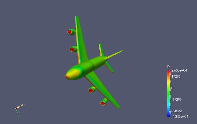
 The pressure plot: The actual influence of the engine in terms of the thrust - is neglected, and so stagnation pressure is observed on the face of the Engines as regions where there is complete deceleration of flow.

 Figure No.2: Pressure Plot

Turbulence Kinetic Energy plot: The k value for the simulation is adopted from the Reynolds number.

U = 230; 

ReL = U*L/nu   % 'L' is the mean aerodynamics Chord length
I=0.16*((ReD)^(-1/8))  % Turbulence Intensity
k = 3/2*(Va*I)^2

                        Figure No.3: Turbulence Kinetic Energy

Velocity Plot: There is deceleration of flow in the wake of the the deflected Elevator tabs.

 Figure No.4: Velocity Plot

Specific dissipation rate: The turbulence dissipation rate is calculated using the following formula. The value is high because a scaled model is used. where the dimensions used for calculating turbulence properties are small.
l=0.07*L;  % L is the mean aerodynamics chord length of the wing
omega = sqrt(k)/(Cm^0.25*l)

Figure No.5: Omega Plot

Residual plot of the flow variables are critical in determining whether the mesh is of good quality and whether or not the simulation results are reliable. 

                                   Figure No.5: Pressure Residual

                                           Figure No.6: Residuals

The residuals suggest that the simulation has converged, this can also be confirmed from the force-Coefficient plots, where the plot has settled down to a specific value. But the value of force-Coefficients, from the above simulation, makes little or no sense because :

1. The actual engine effects are neglected causing large drag values at the engine inlet and
2. The Elevator tab is deflected downwards at high speeds, thus causing a nose pitch down effect and drag.

If the above two factors is considered, a good estimation for force Coefficients can be calculated.