snappyHexMesh Tutorial For a Complex Geometry and External Aerodynamics
The geometry chosen for external fluid dynamics simulation is that of an offshore structure. In that, a deep-draft semi-submersible structure is scaled scaled down to a value of 0.01 (scaled down by a factor of 100). The semi-submersible structures are employed at locations where the oil extraction from the sea bed is considerably deep. These are movable structures which are half submerged during application. A working deck comes right on top of the structure where the cranes and oil rigs are fitted. The semi-submersible consists of four hull appendages which connect the working deck with a pontoon structure. The pontoon structure gives buoyancy to the semi-submersible in deep waters but does not come directly in contact with the ocean bed.

Figure No.1: DDS
The effects of flow induced vibration on the above four columns during high flow currents is indeed the case of interest. Once a good mesh is achieved, the platform is set for the study on the effects of Vortex Induced Vibration and the Vortex Induces Motion. The mesh was created using the snappyHexMesh.
Only some of the key parameters for a complex mesh is addressed in the section. But there is sufficient insight into creating a good Mesh with proper boundary layer addition. The mesh is created for a y+ value less than 1 and the kOmegaSST turbulence model is utilized. The STL file for the semi-submersible structure is created using SolidWorks.


Figure No.2: STL surface and the heading angle
The columns are placed at a 45deg angle to the flow direction as illustrated in the image above. The frontal area is basically the projection area of the submersible which is seen by the incoming flow. This area is important to calculate the force coefficients.

Figure No.3: Projection Area
The STL file is placed inside the constant/triSurface sub-directory and is called inside the background mesh and refined by executing the command 'snappyHexMesh'. The background mesh is created using the blockMeshDict and the cell size in each of the axis direction can be predicted and set depending on the dimension of the geometry and whether or not the STL geometry is scaled.
vertices
(
(-3.0 -3.5 -3.0)
(9.5 -3.5 -3.0)
(9.5 3.5 -3.0)
(-3.0 3.5 -3.0)
(-3.0 -3.5 3.0)
(9.5 -3.5 3.0)
(9.5 3.5 3.0)
(-3.0 3.5 3.0)
);
blocks
(
hex (0 1 2 3 4 5 6 7) (50 28 24) simpleGrading (1 1 1)
);


(
(-3.0 -3.5 -3.0)
(9.5 -3.5 -3.0)
(9.5 3.5 -3.0)
(-3.0 3.5 -3.0)
(-3.0 -3.5 3.0)
(9.5 -3.5 3.0)
(9.5 3.5 3.0)
(-3.0 3.5 3.0)
);
blocks
(
hex (0 1 2 3 4 5 6 7) (50 28 24) simpleGrading (1 1 1)
);
The total co-ordinate length in the X-direction is 12.5(3+9.5). One can chose any of the following cell size (0.1, 0.2, 0.3, 0.4, 0.5, 0.6, 0.7, 0.8, 0.9, 1.0). In the above case a cell size of 0.25 is chosen, and hence the hex number 50 (12.5/0.25). By dividing all the axis lengths by the cell size 0.25, we obtain the following hex cell number (50 28 24). If, for example, one is considering a scaled model whose X directional co-ordinates are between (-0.3 to .95), my cell size will also reduce by a decimal (0.025). A large cell size can be utilized to produce a mesh with y+ value >30 and a smaller cell size for y+ value <1.0.
The surface mesh is created using the STL file -->Surfacesub.stl and a name is assigned to the same. There are also regions within the STL file which can be viewed using Vim editor or the 'gedit' command.
Surfacesub.stl
{
name deepdraft; //name assigned to represent the stl geometry
}
regions
{
deepsemisub //name of the region inside the stl file
{
name appendage; //name assigned to represent the region inside the stl
}
Now to facilitate a proper layer addition, a refinement has to be given to both the stl surface and the region inside the stl file.
deepdraft
{
level (5 6);
regions
{
deepsemisub
{
level (6 7);
patchInfo
{
type wall;
}
}
}
}
By using a coarse background mesh and less refinement we get the following surface mesh:

Figure No.4: Coarse Mesh
Let us now look at an example for a refined surface mesh but inadequate feature snapping. This feature can be controlled by parameters inside the 'surfaceFeatureExtractDict' file and the snapControl parameters inside the snappyHexMeshDict.

Figure No. 5: Bad Feature edge snapping
snapControls
{
nSmoothPatch 3;
tolerance 4.0; //2.0 did not preserve the features. But varies with geometry.
nSolveIter 30; // 300 for good feature snapping after mesh displacement.
nRelaxIter 5;
nFeatureSnapIter 10;
implicitFeatureSnap false;
explicitFeatureSnap true;
multiRegionFeatureSnap false;
}
The two important feature angles inside the snappyHexMeshDict are:
resolveFeatureAngle 30; //Lessr angle would mean more refinement
featureAngle 179; //higher angle would mean good layer extrusion

Figure No.6: Fine surface mesh
We have seen the surface refinement features and now let us move to the region refinement parameters.

Figure No.7: Improper region refinements
The above mesh is a cross-sectional top view, where the sliced view of the pillars are projected. By observation, one can infer the inadequate volume refinement around the pontoons, as also the region between the pontoons in tandem. Good refinement is required to capture the wake effects of the front pontoon on the rear. The volume refinement is achieved through the distance parameter.
refinementRegions
{
deepdraft
{
mode distance;
levels ((0.09 5)); //refinement of level 5 up to 0.09m from surface
}
Everywhere else within the refinement box an arbitrary region refinement is specified.
refinementBox
{
mode inside;
levels ((1E15 4));
}

Figure No.8: Fine Mesh
The Layer addition parameters are listed as follows. Eight layers were added with an expansion ratio of 1.3. The finalLayerThickness is hard to fix for any mesh, but such a low value of 0.17 would only mean that the mesh is refined for a y+ < 1.0. A matlab script can be used to predict the layer thicknesses which is exclusively available on the main page of the blog.
layers
{
"(deepdraft|deepsemisub|appendage).*"
{
nSurfaceLayers 8;
}
}
expansionRatio 1.3;
finalLayerThickness 0.17;
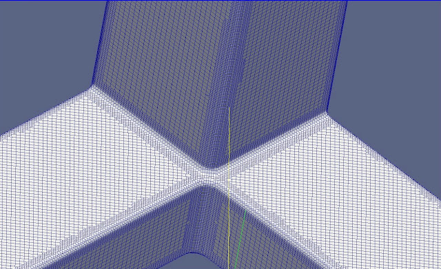
minThickness 0.05;

Figure No.9: Layer Addition and Expansion
One parameter alone was disabled in the mesh quality section, which is key to achieving higher percentage of Layer addition. It is called the minTetQuality and the number of layer addition was reduced to 4 in order to reduce the number cells.
minTetQuality -1; //This parameter is important for boundary layer extrusion


Figure No.10: Mesh Information
Mesh with such low non-orthogonality is required for dynamic mesh simulation.


Here are some of the simulation results.

Figure No.11: Cross-section view vortex shedding

Figure No.12: pimpleFoam results

Figure No.13: simpleFoam results

Figure No.14: Pressure residual


Comments
Post a Comment